LISEM Classic
LISEM
Dynamic Models
With the functionality available in the scripting language, it is possible to write full, fast geo-spatial models. Several convenience functions have been provided for this. Additionally, some usefull physicall processes, such as water flow, have pre-made functions that do most of the work for you.
First, let us make a script where we load an elevation model.
void main()
{
	Map dem = dem.tif;
}
Now, to simulat water flow, we have to make timesteps. We can add a loop that goes through the desired simulation period.
void main()
{
	Map dem = dem.tif;

	//we will simulate 1 hour, with timesteps of 6 seconds.
	int n_steps = 60 *60/6; //nunmber of timesteps
	float t = 0.0; //time in seconds
	float dt = 6.0; //timestep in seconds

	for(int i = 0; i < n_steps; i++)
	{
		t = t + 6;

		//message the user if we are finished another minute
		if( floor(t)%60 == 0)
		{
			Print("We are now at minute : " + ToString(t/60));
		}
	}
}
When you run this script, you should see a message for each minute that passes in the simulation. However, no work is being done yet. To simulate water flow, we will keep track of rainfall. We will simulate a rainfall intensity of 50 mm/hour for the first half hour.
void main()
{
	Map dem = dem.tif;

	//use the elevation model to create an empty map of identical size.
	//this will be the water height, flow velocity in x and y direction
	array<Map> flow = {dem * 0.0,dem * 0.0,dem * 0.0};


	//we will simulate 1 hour, with timesteps of 6 seconds.
	int n_steps = 60 *60/6; //nunmber of timesteps
	float t = 0.0; //time in seconds
	float dt = 6.0; //timestep in seconds
	for(int i = 0; i < n_steps; i++)
	{
		t = t + dt;

		if(t < 30*60)
		{
			//convert to meter/hour
			flow[0] += 50 * dt * 0.001 / (60*60);
		}

        //make a timestep of 6 second with the dynamic flow approximation
        //the resutls overwrites the old data
        flow = FlowDynamic(dem,dem*0.0 + 0.1,flow[0],flow[1],flow[2],6,0.2);

		//message the user if we are finished another minute
		if( floor(t)%60 == 0)
		{
			Print("We are now at minute : " + ToString(t/60));
		}

        //save the model results
	    h_final.tif = flow[0];

	}

}
We can also visualize the result while the model is running. Before the time loop, we add a hillshade map as a background and the initial water height. Then, during the simulation, we keep updating the flow heights.
void main()
{
	Map dem = dem.tif;

	//use the elevation model to create an empty map of identical size.
	//this will be the water height, flow velocity in x and y direction
	array<Map> flow = {dem * 0.0,dem * 0.0,dem * 0.0};

    //add view layers
    AddViewLayer(HillShade(dem),"hillshade");
    UILayer hlay = AddViewLayer(flow[0],"flow height (m)");

	//we will simulate 1 hour, with timesteps of 6 seconds.
	int n_steps = 60 *60/6; //nunmber of timesteps
	float t = 0.0; //time in seconds
	float dt = 6.0; //timestep in seconds
	for(int i = 0; i < n_steps; i++)
	{
		t = t + dt;

		if(t < 30*60)
		{
			//convert to meter/hour
			flow[0] += 50 * dt * 0.001 / (60*60);
		}

        //make a timestep of 6 second with the dynamic flow approximation
        //the resutls overwrites the old data
        flow = FlowDynamic(dem,dem*0.0 + 0.1,flow[0],flow[1],flow[2],6,0.2);

		//message the user if we are finished another minute
		if( floor(t)%60 == 0)
		{
			Print("We are now at minute : " + ToString(t/60));
		}

        //update map viewer
        ReplaceViewLayer(hlay,flow[0]);

        //save the model results
	    h_final.tif = flow[0];

	}

}
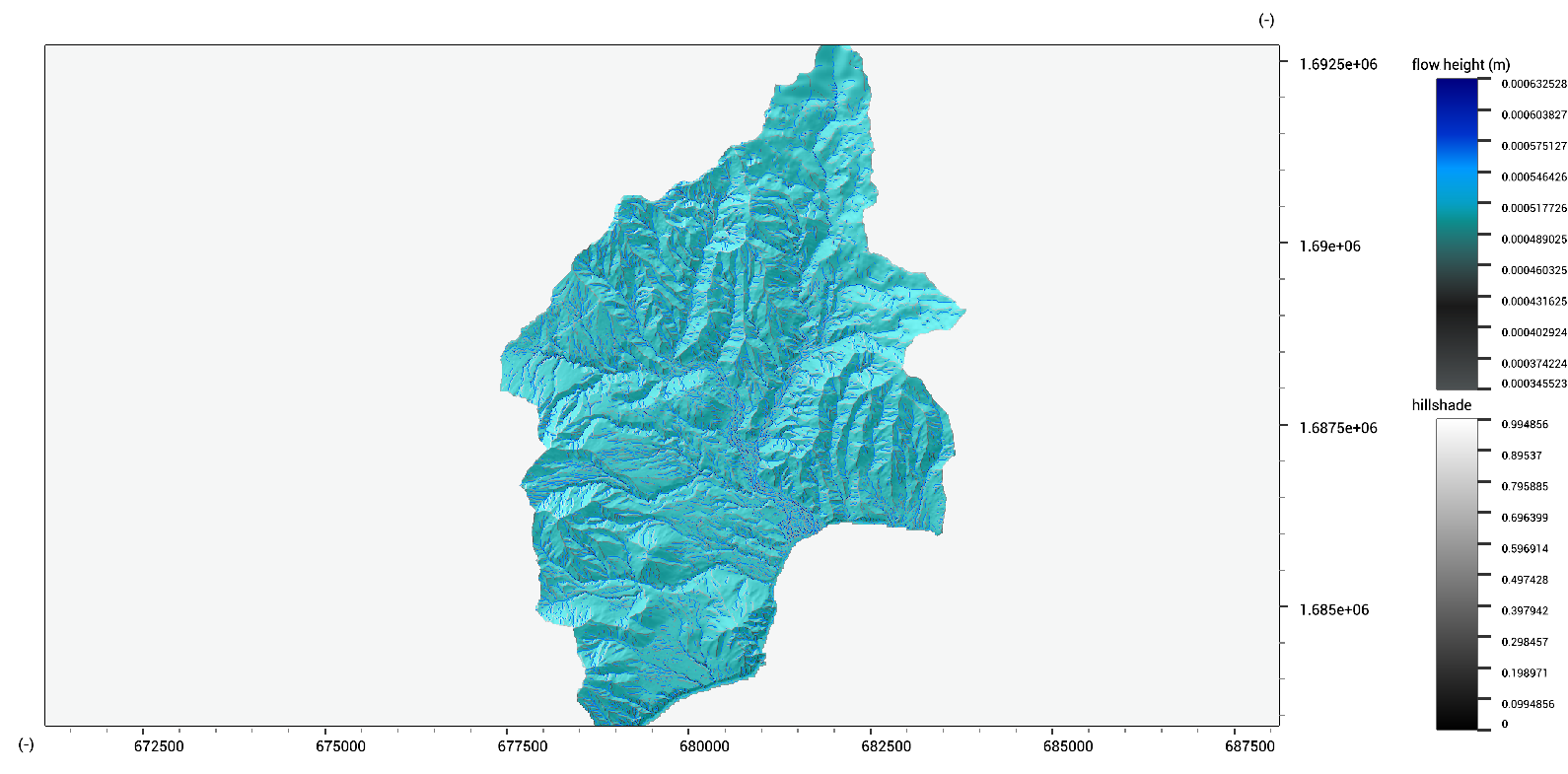
The output to the map viewer can now be seen:
Scripts like these can be easily extended to have specific boundary conditions (incoming waves) or feature additional processes (infiltration, either static or a model such as Green and Ampt).