Hydrology

On this page, running the LISEM model for hydrology will be described. It assumes you have defined your study site and have a decent elevation model for your study site. Additionally, we assume you have a land cover map available. If not, you can use LISEM to classify multi-spectral sattelite imagery such as Sentinel-2, which is freely available at 10 meter spatial resolution.

Data Preparation

Channel properties

If there is a river or channel present in the study site, this can be specified in the model. The flow in such a channel will be simulated as a seperate 1-d water flow, with improved connectivity. Simulating water flow through a channel that is of similar size as the gridcells will usually not work.

Channel locations can be estimated based on drainage patterns. First, we calculate the accuflux based off the drainage network.

accuflux.map = Accuflux(ldd.map,1.0);

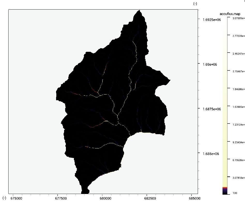
By setting a threshold on the accuflux value, channel cells can automatically be selected. Alternatively, this threshold can also be applied to the stream order (see StreamOrder(LDD)).

channelmask.map = MapIf(accuflux.map >> 5000,1.0,0.0);

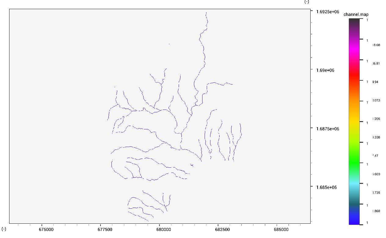
Finally we can take the channel ldd from the main drainage network.

channelldd.map = MapIf(channelmask.map >> 0.5,ldd.map);

The width and depth of the channel might be effectively approximated by one of two methods. First, it is possible to create a custom logarithmic relationship based on the dimensions of the channel at two points. Secondly, but less accurately, global relationships can be used to estimate the dimensions.

channelwidth.tif = 9.68*(accuflux.tif/1e6)**0.32
channeldepth.tif = 11.3*(accuflux.tif/1e6)**0.083

The corrected Channel Mask, Channel LDD, Channel width, Channel depth are available for download.

Land cover properties

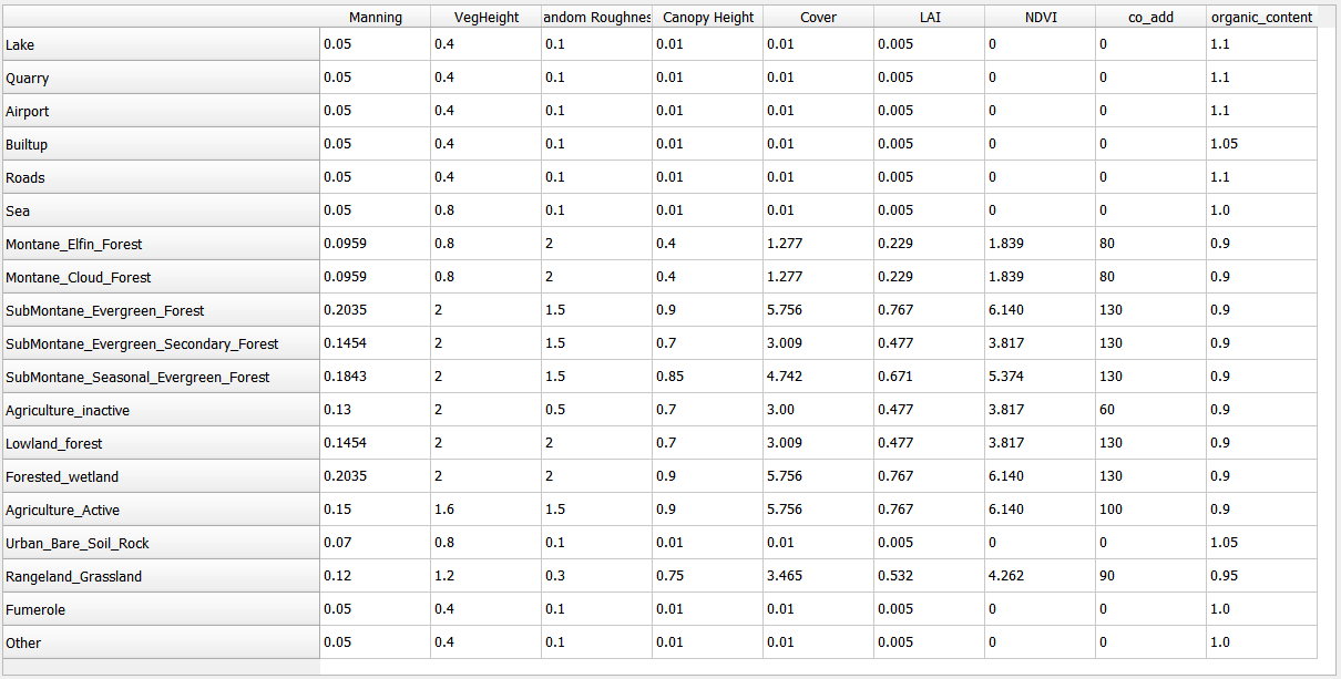
When a land cover map is available, the surface properties can then be defined. The following properties are required:

• Mannings N - estimated through field photos/visits and reference guide such as the USGS field manual for Mannings N
• Vegetation height - estimated through field photos/visits
• Vegetation Cover - estimated through ndvi, or field photos/visits
• SMax Surface - calculated (see below)
• SMax Canopy - calculated (see below)

The first option here is to define these values for each land cover class. You can put these into a table and combine this with the land cover map to create the variable maps. Both are available for download: land use map and lu properties table

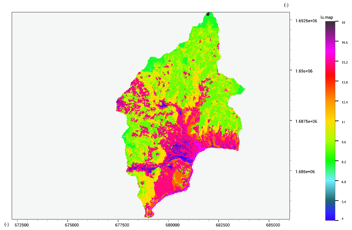
Combining these can be done using the following code:

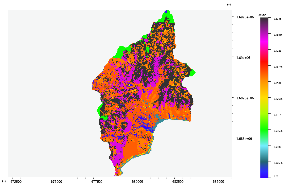
//calculate mannings n
n.tif = RasterFromTable(lu.tbl,lu.map,lu.map * 0.0 + 0);

The second option is to estimate vegetation cover and maximum surface storage from an NDVI (normalized differential vegetation index). Some common emperical relationships are provided below.

• NDVI - NDVI = (NIR-RED)/(NIR+RED) (for sentinel-2 NIR = Band 8, and RED = band 4)
• Vegetation Cover - vegcover=e^((-2.0*NDVI)/(1-NDVI))
• Bare surface Cover - 1.0-vegetation cover
• Leaf area Index - LAI =ln(1-Cover)/(-0.4)
• SMAX Canopy (Crops) - S_max=0.935+0.498 LAI-0.00575 LAI^2
• SMAX Canopy (Pinus) - S_max=0.2331 LAI
• SMAX Canopy (Douglas) - S_max=0.3165 LAI
• SMAX Canopy (Olive) - S_max=1.46 LAI^(0.56 )
• SMAX Canopy (Eucalypt) - S_max=0.0918 LAI^1.04
• SMAX Canopy (Boradleaved Forest) - S_max=0.2856 LAI
• SMAX Canopy (Bracken) - S_max=0.1713 LAI
• SMAX Canopy (Clumped Grass) - S_max=0.59 LAI^0.88
• SMax Surface - S_max=0.243 RR+0.010 RR^2+ 0.012RR S (RR is the standard deviation of the terrain in mm, typically around 2 for roads and around 15 for a forest).

Building elements

You can add building elements to the LISEM simulation by adapting the land use classes to contain buildings and roads. Alternatively, you might add a building cover and road withd map to the simulation. These let LISEM automatically take into account those elements at a sub-pixel level. The building cover is a fraction between 0 (no buildings) and 1 (full building cover). The road witdh indicated the width of a road ina gridcell. This can of course not be more than the width of the gridcell itself. The OpenStreetMaps database is a high-quality open dataset of roads, bridges, buildings and special locations.

Soil properties

Soil properties can be provided through the following inputs, which you can download:

• Clay (fraction between 0 and 1)
• Sand (fraction between 0 and 1)
• Gravel (volumetric fraction)
• Organic Matter (kg per square meter)
• Ground Water Height (m of water height above bed rock)
• Theta Initial (fraction between 0 and 1)

Silt content is assumed to be 1.0 - clay - sand. The initial conditions (ground water height and initial theta) are usually estimated based on antecedent rainfall.

Based on these input paramters, the Saxton et al. (2006) pedotransfer functions are used to estimate saturated conductivity, porosity, field capacity and matric suction. If no measured data is available for these parameters, they can be downloaded from the SOILGRIDS database. If you are interested in checking the values that are calculated by the model, see also the Saxton… Functions in the LISEM scripting environment.

Soil depth

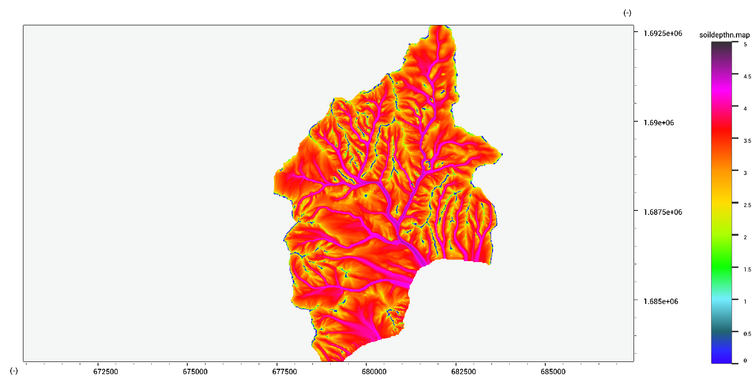
Soil depth is a parameter that is required for hydrology, but is of particular importance to slope stability/failure and ground water flow. In particular as soil depth is critical in Factor of Safety equations. THe actual soil depth varies strongly with slopes, as at any moment, the combination of these two will commonly result in failures if the soil depth becomes too much. As such, inputting soil data that does not consider the variations in slope will result in strange failure patterns. There are several ways in which this difficult parameter might be estimated. The first is the SOILGRIDS database, although the spatial resolution is typically to low for quality results. The second is a physically-based steady state soil depth model. Such a model is provide by lisem:

soildepth.map = AccufluxSoil(dem.map,AccuFlux2D(dem.map,dem.map * 0.0 + 1.0,dem.map * 0.0 + 1.0,500,0.2,1.0),dem.map * 0.0 + 0.001,0.0000001,2,500,0.2);

The results of this model might be calibrated based off measurements of soil depth or of landslide slipe surface depths.

A calibrated version is available to download here. Finally, a multi-variate statistical model might be used, although this is much more site-specific.

Rainfall

Rainfall data can be provided in a simple format.

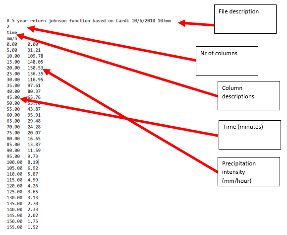
If more complex rainfall input is desired, the values in the file can be replaced with a file name. This file must be a map of same extent as the database, and will be read during the simulation.

Running the model

Running the model can be done from the interface. All the settings can be saved in a runfile. Be sure to save your runfile after providing the desired setting. You can also load existing runfiles.

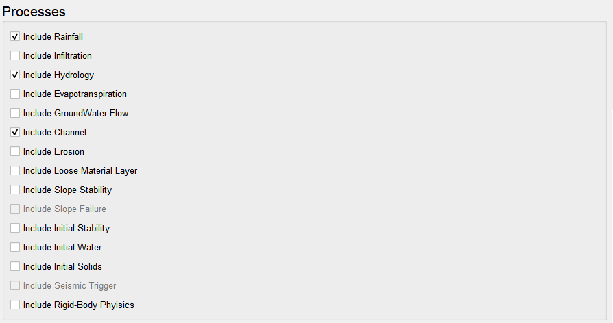
Processes

Select the relevant processes. For now, we simulate rainfall, hydrology, and a channel. Some options depend on other processes (such as slope stabiltiy dpeending on hydrology.

Simulation time domain

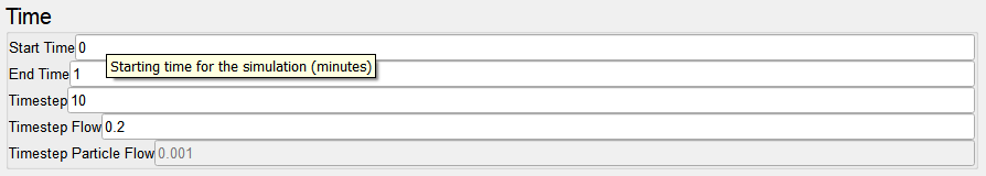
The time settings need to be set to determine the duration of the simulation. Start and end time are in minutes (hold the mouse on the input box to show the tooltip). Timestep and Timestep flow are in seconds. Typically, timestep should be roughly equal to grid cell size. Timestep flow needs to be set low enough to capture the dynamics of flow. The value of 0.2 seconds is a safe default, but for speed increase a higher value (0.5 or 1.0) might be attempted.

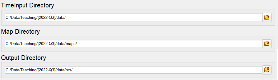
Setting directories

The time input directory will be used to read any time-inputs such as rainfall. Make sure the rainfall.txt file is located in this folder. The map directory must contain all the input maps. Finally, the output directory will be filled with the output maps. Any existing output is overwritten after each timestep.

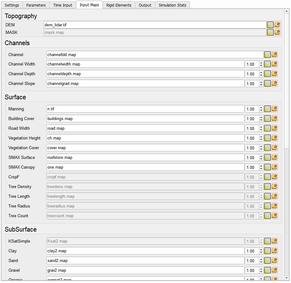
Checking map names

It is usually easiest to provide the maps with their default names, although the names can be changed within the interface. The required maps are highlighted in the list. The numbers after the map act as a multiplier. This can be used for easy calibration.

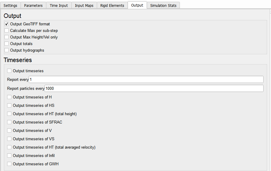
Specifying output

Finally, specify the output options. By default, output is in GeoTIFF format. If this is not checked, the PCRaster-Map format is used. Timeseries can also be written to disk. A list of maps is written for each selected variable. Note that this might quickly fill your hard drive!

Ready, Set, Go!

Finally, remember to save your run-file, and press the play button to start the simulation!

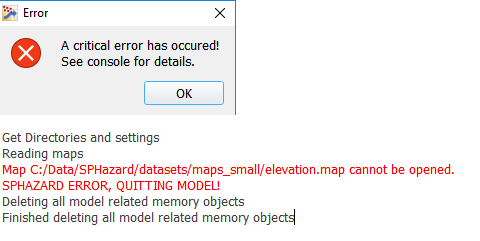
You might get an error message indicating some file was not found. Check the console to see details.

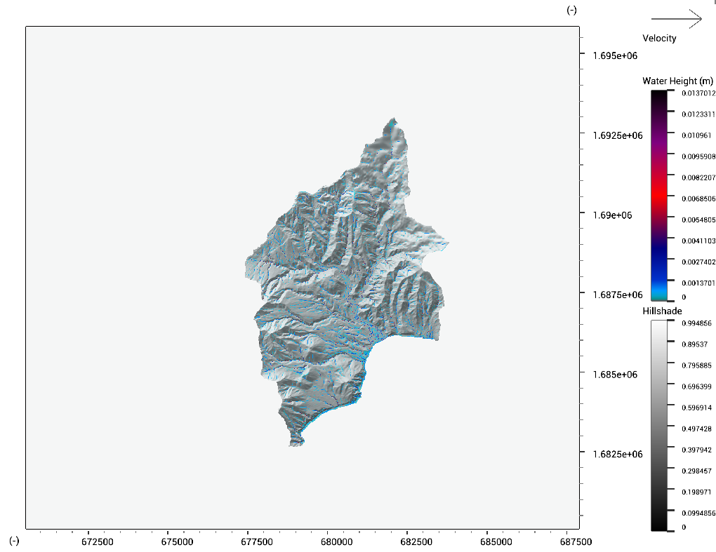
If things worked, you can now see the model in the map viewer.

Initial ground water

The simulation of groundwater dynamics requires the setup of full hydrology. with this aspect working, more processes can be added. Afterwards, the groundwater process can be activated, as it does not require additional data.

Ask a question