Interpolation

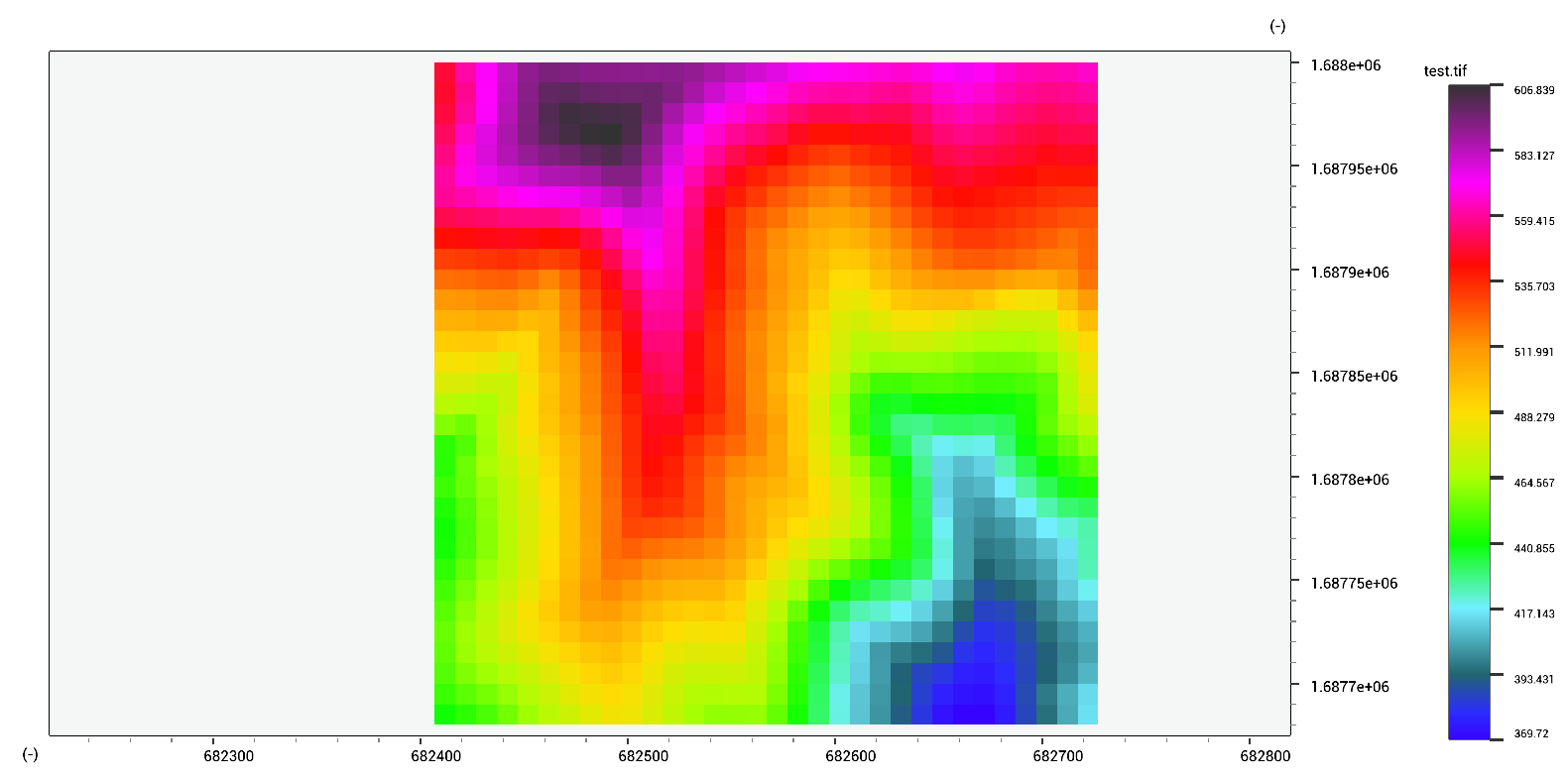
Many types of interpolation are available within LISEM as simple functions. We will be using a small piece of elevation data as a demonstration.

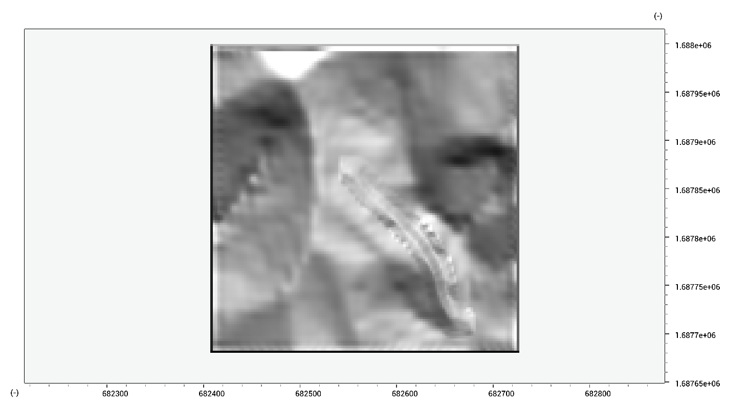
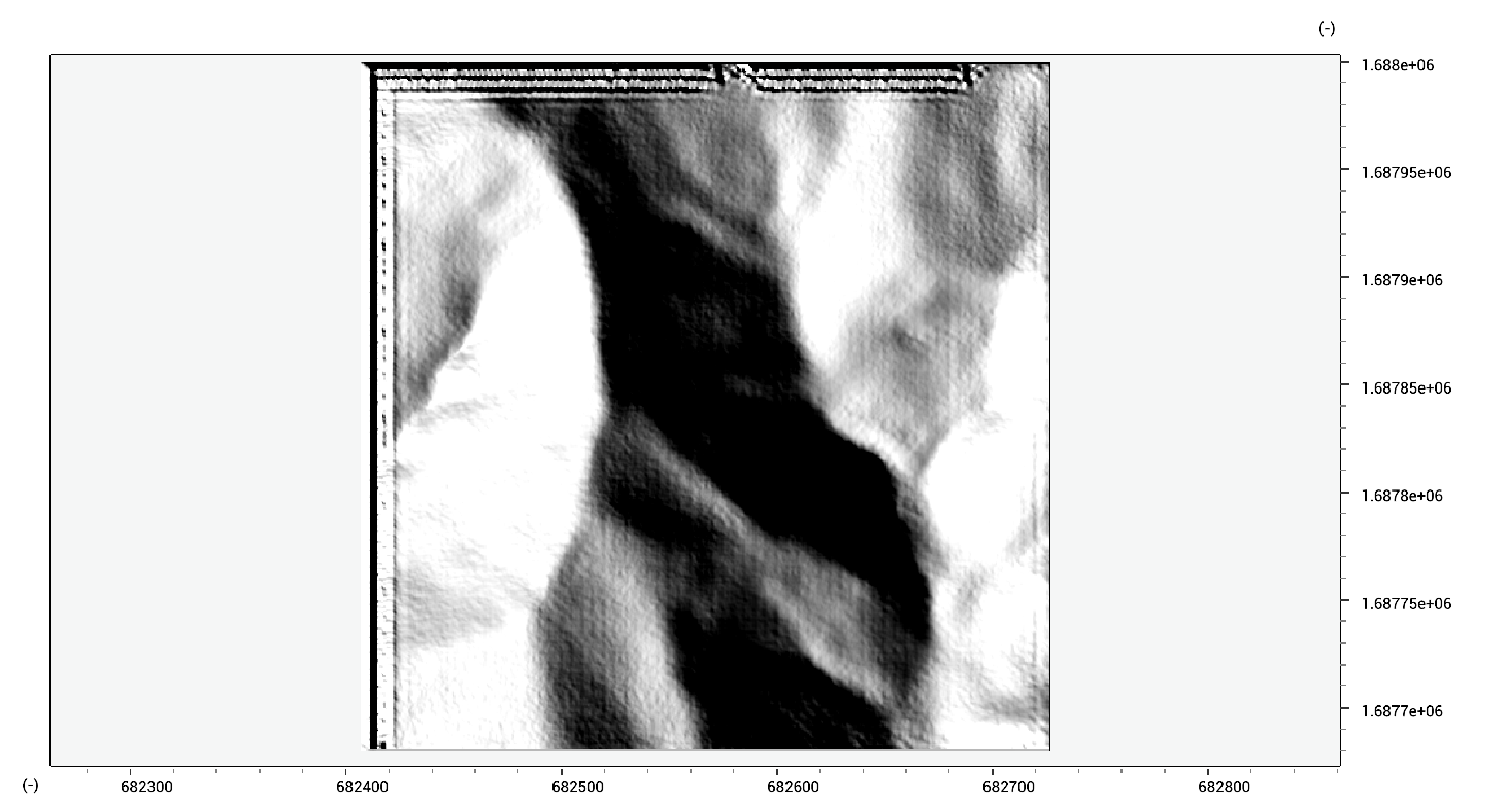
To highlight terrain features, we will look at a shaded relief.

hillshade.tif = HillShade(dem.tif)

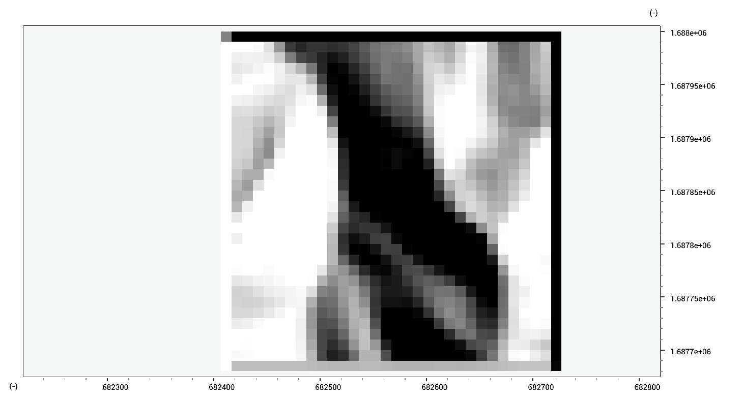
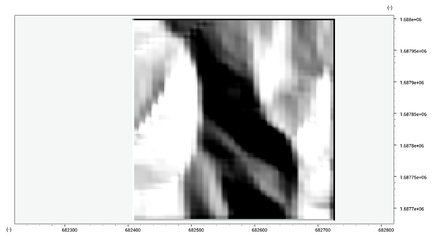
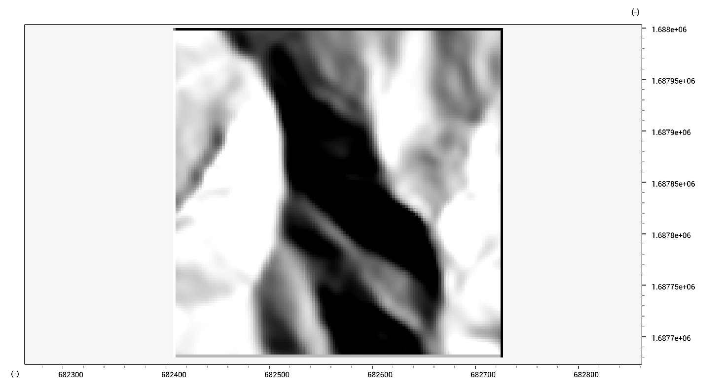
A nearest neighbor interpolation fills in values based on neirest neighbors. The results are shown in hillshaded relief.

nearest.tif = ResampleNearest(dem.tif,4)

These functions can take any scaling number. If larger then 1, it will create higher-resolution data. If smaller then 1, it will create a smaller resolution dataset throuhg averaging.

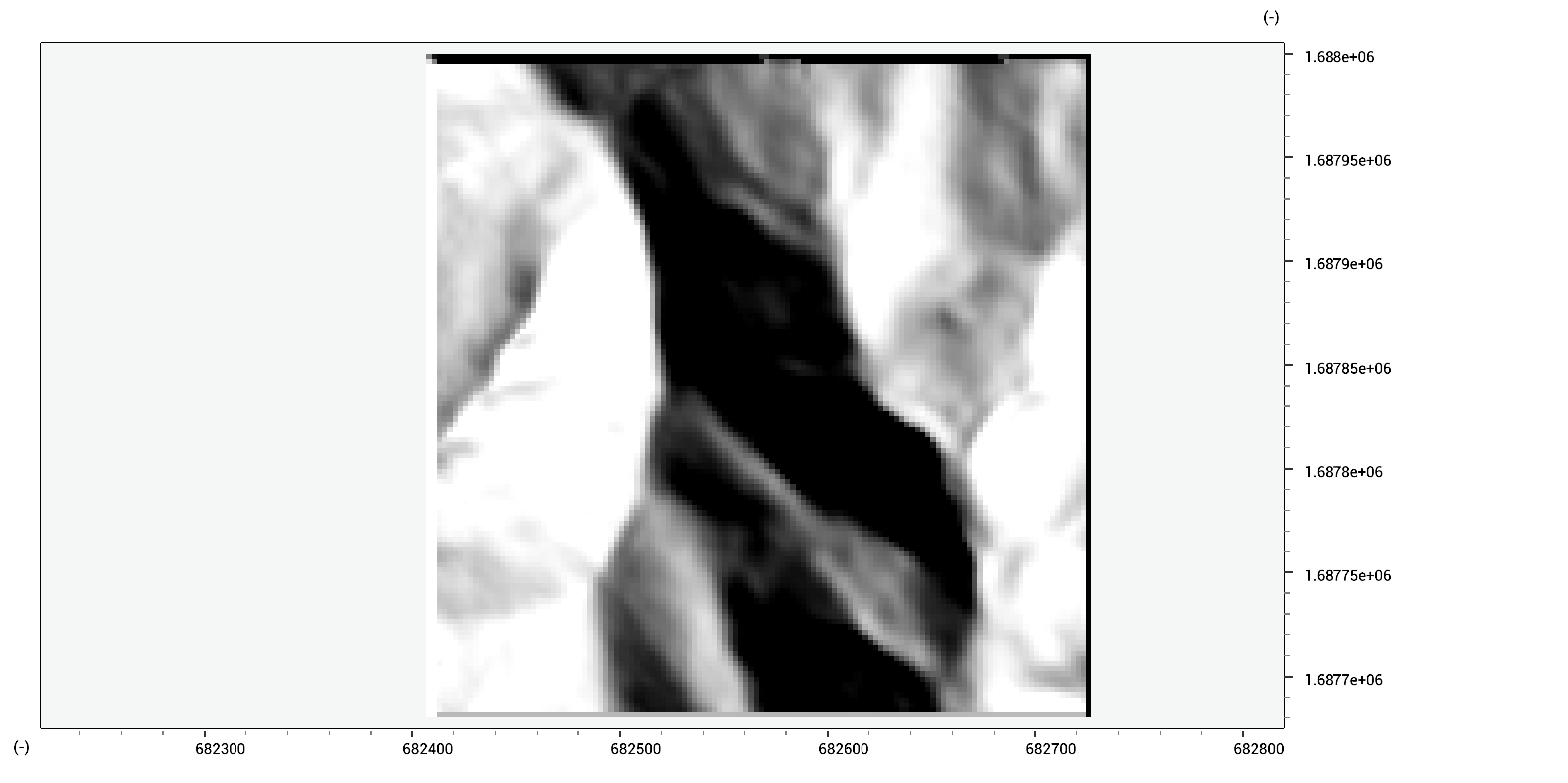
Bilinear interpolation performs better, as its maintains derivatives of the data.

linear.tif = ResampleLinear(dem.tif,4)

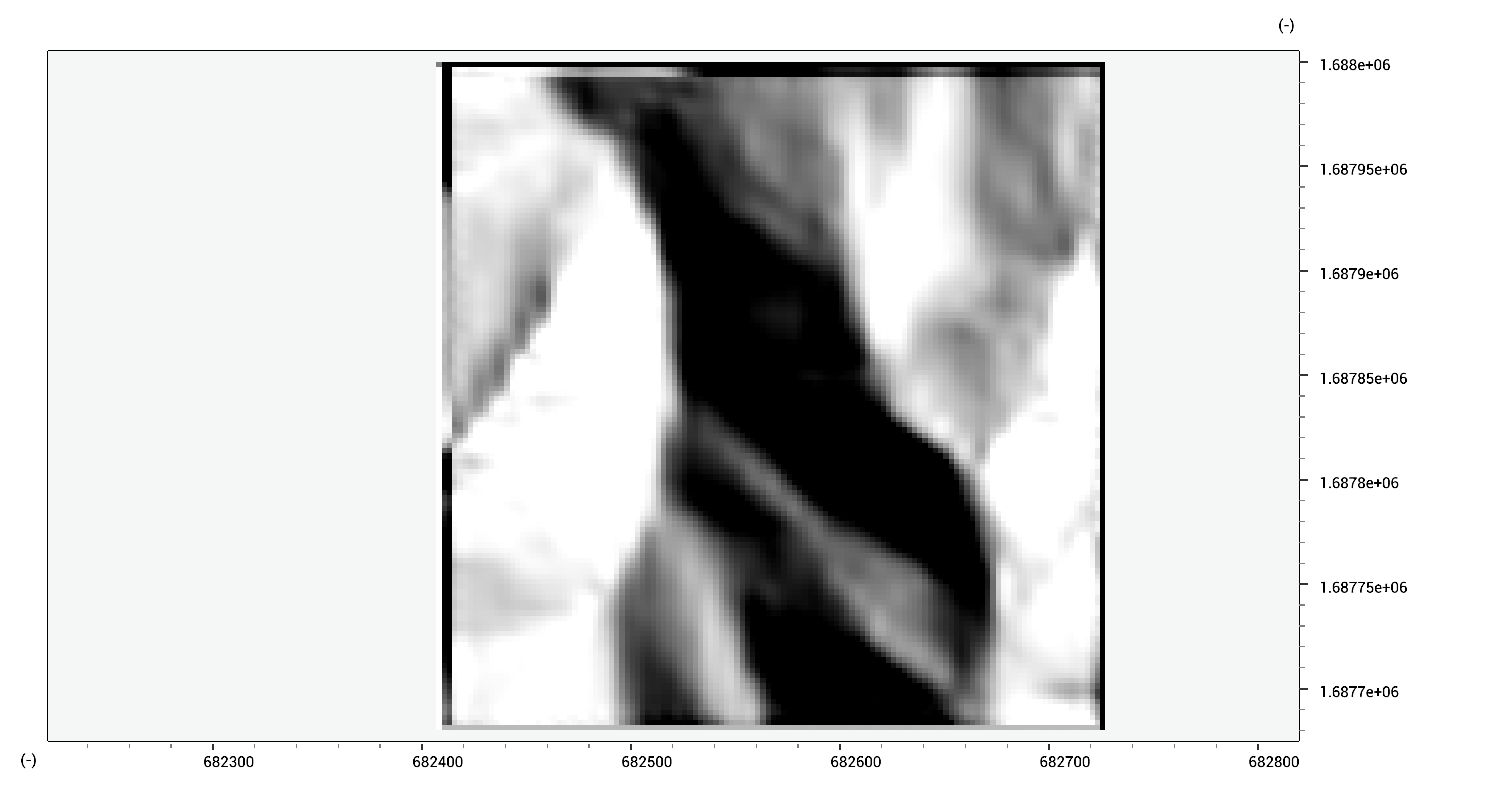
Bicubic interpolation takes into account second derivatives in the data, and thus performs even better.

cubic.tif = ResampleCubic(dem.tif,4)

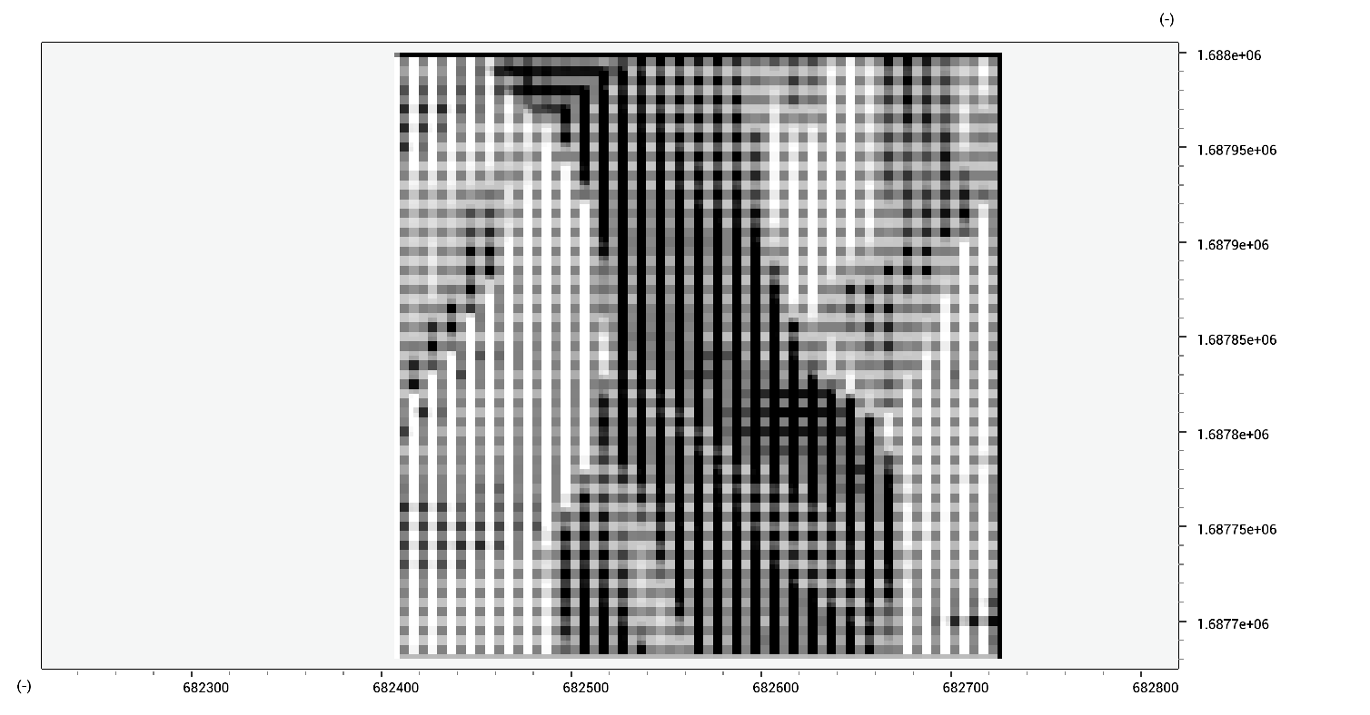
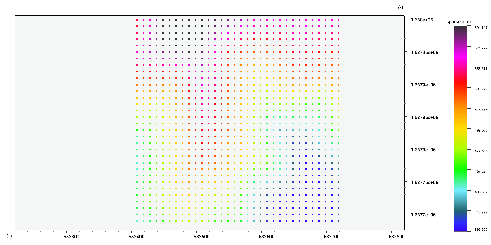
Sparse interpolation provides a means of preparing data for other methods.

sparse.tif = ResampleSparse(dem.tif,4)

A machine learning model can also be applied. Deep neural network machine learning techniques allow for improved interpolation between data. These methods preserive visual detail and can outperform bicubic interpolation by 50 percent. On the downloads page, there is a link to a elevation-data superresolution model (“dahalmodel.onnx”). Using this function (repeatedly) leads to the following produced elevation data.

sr.tif = ApplyMLModel({dem.tif},"DahalModel.onnx",32,32,{0,3,1,2},true)

Applying the model again creates a (4x4) 16 times downscaled dataset. However, artifacts are common in such cases.

sr2.tif = ApplyMLModel({sr.tif},"DahalModel.onnx",32,32,{0,3,1,2},true)

Kriging provides a statistically-sound estimate of the most likely value, but under-estimates variability in the dataset.

kriging.tif = Kriging(sparse.tif,10)

If larger gaps in the data are present, image inpainting techniques can also be used. Telea or Navier-Stokes inpainting are available. In this case, we use a distance of 6, as that is the size of the data gap.

inpaint_telea.tif = InpaintTelea(gap.tif,6)

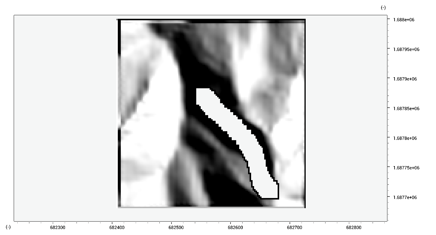
inpaint_ns.tif = InpaintNS(gap.tif,6)

Keep in mind that such results look good in absolute values, but might not perform well on the derivatives of the data.

Ask a question