LISEM Calibration

Calibration and validation is usually required when doing physically-based modelling. In particular for landslide runout and slope failures, uncertainties are many and validation or real events is required to provide the trust in the models capabilities to accurately simulate the dynamics of an event. Calibration means finding the set of input parameters that result in an optimally accurate simulations (in reference to some observed data/event). Validation means to apply a calibrated model blindly (without prior knowledge of the real event) to an event, and assess the accuracy of the prediction. As we have one event, you can carry out calibration and validation using two different locations. However, this means the two sites are highly similar in nature (terrain, geomorphology and geotechnical parameters). So validation will probably be better when compared to validation on a completely different setting.

The first thing to do when calibrating a model, is deciding on a method to calculate the accuracy of the model. There are many metrics designed to do this. If you are considering decimal numbers, the Root Mean Square Error (RSME) might be appropriate. This would work well with flood depths (if you have observed flood depth data to compare to). Other options are the pearson or spearmans correlation indices. In case of discharge, the Nash sutcliffe coefficient can be used. For landslide runout, there is often only an extent available. As such, we need to compare the binary prediction of a model (yes or no impact) with the observations (yes or no impact). This can be done by calculating the percentage of true positive and true negative predictions divided by the total number of pixels. However, this method is biased towards large areas with little landslide activity. Instead, the Cohens Kappa metric provides a correction for this. Take a look at the example Inventory for Grande Bay and Simulated flow for Grande Bay. We can calculate the accuracy as:

double errorval = MapContinuousCohensKappa(inventory.map,impact.map,1.0);
Print("Error is: " + ToString(errorval));

The 1.0 in the code above indicates the critical threshold for defining impact. It is usually not reasonable to define all flow height above 0.0 as impact. In a simulation with hydrology and runoff, all pixels, even with 1 mm of water flow, will be impacted. It is good to think about what the observed data actually is. The inventory consists of mapped impact extends for debris flows and flash floods, but only those that are visible from high resolution sattelite imagery. In this case, we estimated that flow heights above 1.0 left a trace that was distinguishable between the general impact of a tropical cyclone.

We already have seen how to calculate accuracy, while you could manually start changing parameters to find the optimal simulation, there is a more robust way of doing this. Two popular algorithms are: brute-force analysis, and gradient descent. Lets say our model provides an accuracy number, and so acts alittle bit like a function. k=amount of error=f(input parameters) Now, we want to find the input parameters, for which k is at a minimum. Imaging for now, we have one input parameters, cohesion. We could plot our function f, and it might look something like this:

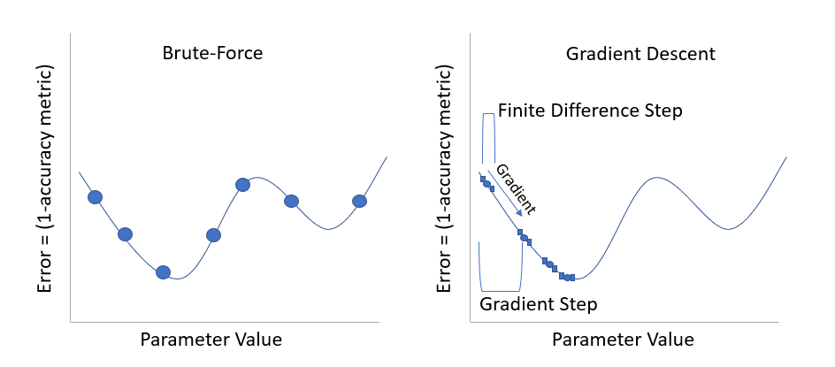
Brute-force analysis attempt to run many different input parameters in a systematic manner, and find the best simulation. Gradient descent attempts to follow the shape of the function f, and steadily descent into a minimum error.

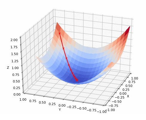
When more parameters are active, gradient descent still works fine, with the exponential increase in required simulations:

Below is a script that shows how to carry out calibration for two parameters (cohesion and internal friction angle) on a simulation with LISEM. There are comments in the script that describe what each line means.

//this function is the error function. It takes a list of parameters (2) and returns the model error 
double Calibrate(array<double> params)
{​​​
	//run the LISEM model, by calling a run file within the working directory.
	//The second argument is a string containing the options is the following format: "name=value|name2=value2"
	//the names can be found within the run-files. Add _cal_mult to a name to get the calibration multiplier.
	//Here, we set the calibration multiplier for internal friction angle and cohesion.
	
	RunModel("run/Couli_AutoCalib.run","Internal Friction Angle_cal_mult="+ToString(params[0])+"|" + "Cohesion Bottom_cal_mult="+ToString(params[1]));


	//load the impact and inventory maps
	Map impact = LoadMap("res/safetyfactor.map");
	Map inventory = 1.0-LoadMap("maps/inventory.tif");
	
	//calculate error value through Cohens Kappa
	double errorval = MapContinuousCohensKappa(inventory,impact,1.0);

	//print info to output window
	Print("Running model with ifa= " + ToString(params[0]) +"& coh= " + ToString(params[1]) + " score = " + ToString(1.0-errorval));

	//actual error is 1.0- Cohens Kappa
	return (1.0-errorval);
}​​​


void main()
{​​​
	//Optimize custom will minimize the error for a function
	//the function Calibrate is defined above
	//we start with two parameters of value 1.0 that must be positive.
	//finite step size = 0.01, gradient step size  = 0.05
	//gradient step size might need to be lowered for stable convergence.
	OptimizeCustom({​​​1.0,1.0}​​​,{​​​true,true}​​​,@Calibrate,0.01,0.05);
}​​​

Typically, the script will require some 30 iterations for a 2 or 3 parameter calibration. Do check the result in the display to alter the gradient step if neccesary.

Ask a question